List of Machine Learning Approaches
List of ML Approaches
- This is a reference list of tools and methods for solving various ML problems
Probabilistic Modeling
Naive Bayes algorithm
- Assumes all the input features are independent from each other
In spite of their apparently over-simplified assumptions, naive Bayes classifiers have worked quite well in many real-world situations, famously document classification and spam filtering. They require a small amount of training data to estimate the necessary parameters. (For theoretical reasons why naive Bayes works well, and on which types of data it does, see the references below.)
Naive Bayes learners and classifiers can be extremely fast compared to more sophisticated methods. The decoupling of the class conditional feature distributions means that each distribution can be independently estimated as a one dimensional distribution. This in turn helps to alleviate problems stemming from the curse of dimensionality.
On the flip side, although naive Bayes is known as a decent classifier, it is known to be a bad estimator, so the probability outputs from predict_proba are not to be taken too seriously.
from sklearn.datasets import load_iris
from sklearn.model_selection import train_test_split
from sklearn.naive_bayes import GaussianNB
X, y = load_iris(return_X_y=True)
X_train, X_test, y_train, y_test = train_test_split(X, y, test_size=0.5, random_state=0)
gnb = GaussianNB()
y_pred = gnb.fit(X_train, y_train).predict(X_test)
print("Number of mislabeled points out of a total %d points : %d"
      % (X_test.shape[0], (y_test != y_pred).sum()))
Number of mislabeled points out of a total 75 points : 4
Logistic Regression (logreg)
- Classification not a regression algorithm (cat vs. dog not 3 bananas vs. 10 bananas)
from sklearn.datasets import load_iris
from sklearn.linear_model import LogisticRegression
X, y = load_iris(return_X_y=True)
clf = LogisticRegression(random_state=0).fit(X, y)
clf.predict(X[:2, :])
C:\Users\rober\anaconda3\envs\deep-learning-book\lib\site-packages\sklearn\linear_model\_logistic.py:814: ConvergenceWarning: lbfgs failed to converge (status=1):
STOP: TOTAL NO. of ITERATIONS REACHED LIMIT.

Increase the number of iterations (max_iter) or scale the data as shown in:
    https://scikit-learn.org/stable/modules/preprocessing.html
Please also refer to the documentation for alternative solver options:
    https://scikit-learn.org/stable/modules/linear_model.html#logistic-regression
  n_iter_i = _check_optimize_result(


array([0, 0])
clf.predict_proba(X[:2, :])
array([[9.81797141e-01, 1.82028445e-02, 1.44269293e-08],
       [9.71725476e-01, 2.82744937e-02, 3.01659208e-08]])
clf.score(X, y)
0.9733333333333334
Kernel Methods
Support Vector Machines (SVM)
Can be used for multiple approaches:
- Classification,
- Regression
- Outliers detection.
The advantages of support vector machines are:
- Effective in high dimensional spaces.
- Still effective in cases where number of dimensions is greater than the number of samples.
- Uses a subset of training points in the decision function (called support vectors), so it is also memory efficient.
- Versatile: different Kernel functions can be specified for the decision function. Common kernels are provided, but it is also possible to specify custom kernels.
The disadvantages of support vector machines include:
If the number of features is much greater than the number of samples, avoid over-fitting in choosing Kernel functions and regularization term is crucial.
SVMs do not directly provide probability estimates, these are calculated using an expensive five-fold cross-validation (see Scores and probabilities, below).
The support vector machines in scikit-learn support both dense (numpy.ndarray and convertible to that by numpy.asarray) and sparse (any scipy.sparse) sample vectors as input. However, to use an SVM to make predictions for sparse data, it must have been fit on such data. For optimal performance, use C-ordered numpy.ndarray (dense) or scipy.sparse.csr_matrix (sparse) with dtype=float64.
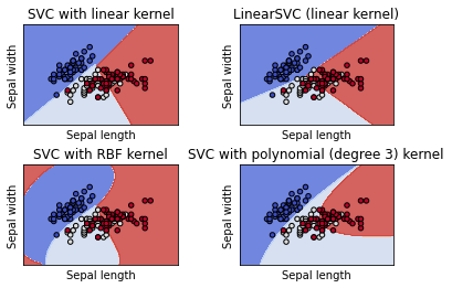
SVM is a classification algorithm that works by finding “decision boundaries” separating two classes. SVMs proceed to find these boundaries in two steps:
The data is mapped to a new high-dimensional representation where the decision boundary can be expressed as a hyperplane (if the data was two-dimensional, a hyperplane would be a straight line, in 3D, it would be a 2D plane). A good decision boundary (a separation hyperplane) is computed by trying to maximize the distance between the hyperplane and the closest data points from each class, a step called maximizing the margin. This allows the boundary to generalize well to new samples outside of the training dataset.
- SVMs aren’t good for large datasets
import numpy as np
import matplotlib.pyplot as plt
from sklearn import svm, datasets


def make_meshgrid(x, y, h=0.02):
    """Create a mesh of points to plot in

    Parameters
    ----------
    x: data to base x-axis meshgrid on
    y: data to base y-axis meshgrid on
    h: stepsize for meshgrid, optional

    Returns
    -------
    xx, yy : ndarray
    """
    x_min, x_max = x.min() - 1, x.max() + 1
    y_min, y_max = y.min() - 1, y.max() + 1
    xx, yy = np.meshgrid(np.arange(x_min, x_max, h), np.arange(y_min, y_max, h))
    return xx, yy


def plot_contours(ax, clf, xx, yy, **params):
    """Plot the decision boundaries for a classifier.

    Parameters
    ----------
    ax: matplotlib axes object
    clf: a classifier
    xx: meshgrid ndarray
    yy: meshgrid ndarray
    params: dictionary of params to pass to contourf, optional
    """
    Z = clf.predict(np.c_[xx.ravel(), yy.ravel()])
    Z = Z.reshape(xx.shape)
    out = ax.contourf(xx, yy, Z, **params)
    return out


# import some data to play with
iris = datasets.load_iris()
# Take the first two features. We could avoid this by using a two-dim dataset
X = iris.data[:, :2]
y = iris.target

# we create an instance of SVM and fit out data. We do not scale our
# data since we want to plot the support vectors
C = 1.0  # SVM regularization parameter
models = (
    svm.SVC(kernel="linear", C=C),
    svm.LinearSVC(C=C, max_iter=10000),
    svm.SVC(kernel="rbf", gamma=0.7, C=C),
    svm.SVC(kernel="poly", degree=3, gamma="auto", C=C),
)
models = (clf.fit(X, y) for clf in models)

# title for the plots
titles = (
    "SVC with linear kernel",
    "LinearSVC (linear kernel)",
    "SVC with RBF kernel",
    "SVC with polynomial (degree 3) kernel",
)

# Set-up 2x2 grid for plotting.
fig, sub = plt.subplots(2, 2)
plt.subplots_adjust(wspace=0.4, hspace=0.4)

X0, X1 = X[:, 0], X[:, 1]
xx, yy = make_meshgrid(X0, X1)

for clf, title, ax in zip(models, titles, sub.flatten()):
    plot_contours(ax, clf, xx, yy, cmap=plt.cm.coolwarm, alpha=0.8)
    ax.scatter(X0, X1, c=y, cmap=plt.cm.coolwarm, s=20, edgecolors="k")
    ax.set_xlim(xx.min(), xx.max())
    ax.set_ylim(yy.min(), yy.max())
    ax.set_xlabel("Sepal length")
    ax.set_ylabel("Sepal width")
    ax.set_xticks(())
    ax.set_yticks(())
    ax.set_title(title)

plt.show()
Decision Trees, Random Forests, Gradient Boosting Machines
Decision Trees
-
Classification and Regression
-
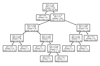
Decision trees are flowchart-like structures that let you classify input data points or predict output values given inputs. They’re easy to visualize and interpret.
Classification
from sklearn.datasets import load_iris
from sklearn import tree
from sklearn.tree import export_text

iris = load_iris()
X, y = iris.data, iris.target
clf = tree.DecisionTreeClassifier()
clf = clf.fit(X, y)
tree.plot_tree(clf)
r = export_text(clf, feature_names=iris['feature_names'])
print(r)
|--- petal width (cm) <= 0.80
|   |--- class: 0
|--- petal width (cm) >  0.80
|   |--- petal width (cm) <= 1.75
|   |   |--- petal length (cm) <= 4.95
|   |   |   |--- petal width (cm) <= 1.65
|   |   |   |   |--- class: 1
|   |   |   |--- petal width (cm) >  1.65
|   |   |   |   |--- class: 2
|   |   |--- petal length (cm) >  4.95
|   |   |   |--- petal width (cm) <= 1.55
|   |   |   |   |--- class: 2
|   |   |   |--- petal width (cm) >  1.55
|   |   |   |   |--- petal length (cm) <= 5.45
|   |   |   |   |   |--- class: 1
|   |   |   |   |--- petal length (cm) >  5.45
|   |   |   |   |   |--- class: 2
|   |--- petal width (cm) >  1.75
|   |   |--- petal length (cm) <= 4.85
|   |   |   |--- sepal width (cm) <= 3.10
|   |   |   |   |--- class: 2
|   |   |   |--- sepal width (cm) >  3.10
|   |   |   |   |--- class: 1
|   |   |--- petal length (cm) >  4.85
|   |   |   |--- class: 2
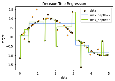
Regression
# Import the necessary modules and libraries
import numpy as np
from sklearn.tree import DecisionTreeRegressor
import matplotlib.pyplot as plt

# Create a random dataset
rng = np.random.RandomState(1)
X = np.sort(5 * rng.rand(80, 1), axis=0)
y = np.sin(X).ravel()
y[::5] += 3 * (0.5 - rng.rand(16))

# Fit regression model
regr_1 = DecisionTreeRegressor(max_depth=2)
regr_2 = DecisionTreeRegressor(max_depth=5)
regr_1.fit(X, y)
regr_2.fit(X, y)

# Predict
X_test = np.arange(0.0, 5.0, 0.01)[:, np.newaxis]
y_1 = regr_1.predict(X_test)
y_2 = regr_2.predict(X_test)

# Plot the results
plt.figure()
plt.scatter(X, y, s=20, edgecolor="black", c="darkorange", label="data")
plt.plot(X_test, y_1, color="cornflowerblue", label="max_depth=2", linewidth=2)
plt.plot(X_test, y_2, color="yellowgreen", label="max_depth=5", linewidth=2)
plt.xlabel("data")
plt.ylabel("target")
plt.title("Decision Tree Regression")
plt.legend()
plt.show()
Random Forests
- Based on randomized ensembles of the previous decision trees
from sklearn.model_selection import cross_val_score
from sklearn.datasets import make_blobs
from sklearn.ensemble import RandomForestClassifier
from sklearn.ensemble import ExtraTreesClassifier
from sklearn.tree import DecisionTreeClassifier

X, y = make_blobs(n_samples=10000, n_features=10, centers=100, random_state=0)

clf = DecisionTreeClassifier(max_depth=None, min_samples_split=2, random_state=0)
scores = cross_val_score(clf, X, y, cv=5)
scores.mean()
0.9823000000000001
clf = RandomForestClassifier(n_estimators=10, max_depth=None, min_samples_split=2, random_state=0)
scores = cross_val_score(clf, X, y, cv=5)
scores.mean()
0.9997
clf = ExtraTreesClassifier(n_estimators=10, max_depth=None, min_samples_split=2, random_state=0)
scores = cross_val_score(clf, X, y, cv=5)
scores.mean()
1.0
Gradient Boosting Machines
Nice Post on Gradient Boosting
A gradient boosting machine, much like a random forest, is a machine learning technique based on ensembling weak prediction models, generally decision trees. It uses gradient boosting, a way to improve any machine learning model by iteratively training new models that specialize in addressing the weak points of the previous models. Applied to decision trees, the use of the gradient boosting technique results in models that strictly outperform random forests most of the time, while having similar properties. It may be one of the best, if not the best, algorithm for dealing with nonperceptual data today. Alongside deep learning, it’s one of the most commonly used techniques in Kaggle competitions.
from sklearn.datasets import make_hastie_10_2
from sklearn.ensemble import GradientBoostingClassifier

X, y = make_hastie_10_2(random_state=0)
X_train, X_test = X[:2000], X[2000:]
y_train, y_test = y[:2000], y[2000:]
clf = GradientBoostingClassifier(n_estimators=100, learning_rate=1.0, max_depth=1, random_state=0).fit(X_train, y_train)
clf.score(X_test, y_test)
0.913
The two techniques you should be familiar with in order to be successful in applied machine learning are gradient boosted trees, for shallow-learning problems; and deep learning, for perceptual problems.
These can be implemented with with Scikit-learn, XGBoost, and Keras—the three libraries that currently dominate Kaggle competitions.
## Long Short-Term Memory (LSTM) algorithm
- Fundamental to deep learning for timeseries
## Computer vision
- ResNet,
- Inception
- Xception
Natural Language Processing (NLP)
- large Transformer-based architectures such as
- BERT,
- GPT-3
- XLNet