Deep Learning Part 2 Neural Net Math

The mathematical building blocks of neural networks

This chapter covers

• A first example of a neural network
• Tensors and tensor operations
• How neural networks learn via backpropagation and gradient descent

This will be the second part of a series of posts for my own reference and continued professional development in deep learning. It should mostly follow important points taken from François Chollet’s book Deep Learning with Python, Second Edition.

The main book itself can be found at Manning.com

#Running a custom runtime with anaconda

#(base) conda install nb_conda_kernels
# conda create --name deep-learning
# conda activate deep-learning
# conda install ipykernel
# conda install tensorflow==2.6 keras==2.6

#Here in Jupyter, menu>Kernel>Change kernel>conda env:deep-learning

• MNIST dataset (Modified National Institute of Standards and Technology) is the “Hello World” of neural networks and machine learning.

• Deep learning requires familiarity with:

  • tensors,
  • tensor operations
  • differentiation
  • gradient descent

A first look at a neural network

The MNIST dataset is a series of handwritten digits, digitized into 28x28 grayscale images and appropriately classified from 0 to 9. We’re going to make a basic network to classify them.

Loading the MNIST dataset in Keras

from tensorflow.keras.datasets import mnist
import numpy as np

#standard syntax for keras datasets
(train_images, train_labels), (test_images, test_labels) = mnist.load_data()
(train_images_2, train_labels_2), (test_images_2, test_labels_2) = mnist.load_data()

#how many dimensions?
train_images.shape

(60000, 28, 28)

There are 60,000 training examples, each 28 by 28 pixels

len(train_labels)

60000

Good data should have the same number of labels as training examples

train_labels

array([5, 0, 4, ..., 5, 6, 8], dtype=uint8)

test_images.shape

(10000, 28, 28)

Now we know we have 10K testing images. This is similar to a standard 80/20 or 90/10 test split but it’s more like a 15% test split.

len(test_labels)

10000

test_labels

array([7, 2, 1, ..., 4, 5, 6], dtype=uint8)

The network architecture

Two dense layers (also called fully connected) will be the basis of the neural architecture. Their job is to extract more useful representations of the data into a distilled version of the information. This data distillation is both a means of extracting information from the input and a form of data compression for free!

from tensorflow import keras
from tensorflow.keras import layers

#Very Simple initial architecture - 512 nodes on the first layer, 
#10 output nodes on the second layer.
model = keras.Sequential([
    layers.Dense(512, activation="relu"),
    layers.Dense(10, activation="softmax")
])

The compilation step

Compilation requires three more steps:

• An optimizer
• A loss function
• Metrics to monitor during training and testing

# A lot of options are possible here but this is pretty standard for this type of job. 
model.compile(optimizer="rmsprop",
              loss="sparse_categorical_crossentropy",
              metrics=["accuracy"])

Preparing the image data

• Turn each image into a single vector to be shown to the network
• normalize each grayscale number from its 0-255 range (uint8 data type) to 0 to 1 (float32)

train_images = train_images.reshape((60000, 28 * 28))
train_images = train_images.astype("float32") / 255
test_images = test_images.reshape((10000, 28 * 28))
test_images = test_images.astype("float32") / 255

“Fitting” the model

the [model].fit([parameters]) syntax is consistent throughout Keras and scikit-learn

model.fit(train_images, train_labels, epochs=5, batch_size=128)

Epoch 1/5
469/469 [==============================] - 2s 3ms/step - loss: 0.2579 - accuracy: 0.9254
Epoch 2/5
469/469 [==============================] - 2s 3ms/step - loss: 0.1049 - accuracy: 0.9691
Epoch 3/5
469/469 [==============================] - 1s 3ms/step - loss: 0.0695 - accuracy: 0.9793
Epoch 4/5
469/469 [==============================] - 1s 3ms/step - loss: 0.0502 - accuracy: 0.9848
Epoch 5/5
469/469 [==============================] - 1s 3ms/step - loss: 0.0377 - accuracy: 0.9888





<keras.callbacks.History at 0x21965d9e190>

The final accuracy was 98.9%

Using the model to make predictions

Now that the model has been trained via the .fit method, we can now use the model and it’s associated parameters/weights to predict new samples.

test_digits = test_images[0:10]
predictions = model.predict(test_digits)
predictions[0]

array([1.2659244e-10, 4.6564801e-11, 9.7060592e-07, 4.3473542e-06,
       7.4439471e-14, 1.4966636e-08, 2.5408643e-16, 9.9999452e-01,
       5.4953309e-09, 1.7923185e-07], dtype=float32)

predictions is now an array of arrays, each element of the highest level array has the probability for each number held within a 10-element array. To find the predicted number, we find the index of the maximum value via the .argmax() method.

predictions[0].argmax()

7

So now we can compare the two cases between the predicted value (7) vs. the correct label for that datapoint.

predictions[0][7]

0.9999945

test_labels[0]

7

The two are the same!

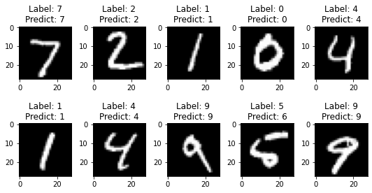
We can now plot the first ten test items along with their predictions.

import matplotlib.pyplot as plt
num = 10
images = test_images_2[:num]
labels = test_labels_2[:num]

predictions = model.predict(images.reshape((num, 28 * 28)))

num_row = 2
num_col = 5# plot images
fig, axes = plt.subplots(num_row, num_col, figsize=(1.5*num_col,2*num_row))
for i in range(num):
    ax = axes[i//num_col, i%num_col]
    ax.imshow(images[i], cmap='gray')
    ax.set_title('Label: {}\nPredict: {}'.format(labels[i], predictions[i].argmax()))
plt.tight_layout()
plt.show()

Find examples where it predicted wrong and visualize them

# Make predictions for every test image
all_predictions = model.predict(test_images.reshape((10000, 28 * 28)))

#grab the images where the predictions don't match the label
predicted_labels = np.argmax(all_predictions, axis=1)
failed_items = np.not_equal(predicted_labels,test_labels)
test_fails = test_images[failed_items]

#same indices used for predictions and labels 
prediction_fails = predicted_labels[failed_items]
label_fails = test_labels[failed_items]

num = 50

num_row = 5
num_col = 10# plot images
fig, axes = plt.subplots(num_row, num_col, figsize=(1.5*num_col,2*num_row))
for i in range(num):
    ax = axes[i//num_col, i%num_col]
    ax.imshow(test_fails[i].reshape(28, 28), cmap='gray')
    ax.set_title('Label: {}\nPredict: {}'.format(label_fails[i], prediction_fails[i]))
plt.tight_layout()
plt.show()

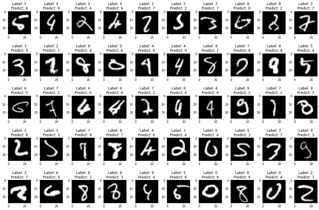
Getting into these failures can help to diagnose and direct next steps for improving the algorithm.

Some of these example look very difficult!

Evaluating the model on new data

Get the accuracy rates for the full 10k test images.

test_loss, test_acc = model.evaluate(test_images, test_labels)
print(f"test_acc: {test_acc}")

313/313 [==============================] - 0s 873us/step - loss: 0.0699 - accuracy: 0.9796
test_acc: 0.9796000123023987

If we compare this accuracy on the test set vs. the training set, we got 97.92% on this whereas we scored 98.9% on the training data. This is a textbook example of the system overfitting onto the training data. More on overfitting will be in the next part.

Let’s do it again but show the accuracies with a graph. You’ll note the accuracy on the validation set from the overfitting doesn’t improve nearly as quickly which could be improved with a dropout layer.

import tensorflow as tf

# Load the TensorBoard notebook extension
%load_ext tensorboard
import datetime

def create_model():
  return tf.keras.models.Sequential([
    tf.keras.layers.Flatten(input_shape=(28, 28)),
    tf.keras.layers.Dense(512, activation='relu'),
    tf.keras.layers.Dense(10, activation='softmax')
  ])

(x_train, y_train),(x_test, y_test) = mnist.load_data()
x_train, x_test = x_train / 255.0, x_test / 255.0

model = create_model()
model.compile(optimizer='adam',
              loss='sparse_categorical_crossentropy',
              metrics=['accuracy'])

log_dir = "logs/fit/" + datetime.datetime.now().strftime("%Y%m%d-%H%M%S")
tensorboard_callback = tf.keras.callbacks.TensorBoard(log_dir=log_dir, histogram_freq=1)

model.fit(x=x_train, 
          y=y_train, 
          epochs=5, 
          validation_data=(x_test, y_test), 
          callbacks=[tensorboard_callback])

%tensorboard --logdir logs/fit

Epoch 1/5
1875/1875 [==============================] - 4s 2ms/step - loss: 0.2026 - accuracy: 0.9409 - val_loss: 0.1076 - val_accuracy: 0.9651
Epoch 2/5
1875/1875 [==============================] - 3s 2ms/step - loss: 0.0802 - accuracy: 0.9750 - val_loss: 0.0797 - val_accuracy: 0.9762
Epoch 3/5
1875/1875 [==============================] - 3s 2ms/step - loss: 0.0517 - accuracy: 0.9838 - val_loss: 0.0726 - val_accuracy: 0.9782
Epoch 4/5
1875/1875 [==============================] - 3s 2ms/step - loss: 0.0365 - accuracy: 0.9886 - val_loss: 0.0767 - val_accuracy: 0.9789
Epoch 5/5
1875/1875 [==============================] - 3s 2ms/step - loss: 0.0276 - accuracy: 0.9909 - val_loss: 0.0726 - val_accuracy: 0.9791



Reusing TensorBoard on port 6006 (pid 7236), started 1:16:58 ago. (Use '!kill 7236' to kill it.)

Next we’ll learn about tensors, tensor operations, and gradient descent.

Data representations for neural networks

An array of (usually) numbers (such as the numpy arrays above) is called a tensor.

The dimensionality of the tensor gives its rank and lower rank tensors have common names:

• Rank-0 tensor (single number) is a constant
• Rank-1 tensor (list or column) is a vector
• Rank-2 tensor (table) is a matrix

In the context of tensors, a dimension is typically called an axis.

Scalars (rank-0 tensors)

single number as an array

import numpy as np
x = np.array(12)
x

array(12)

#number of dimensions of the array
x.ndim

0

Vectors (rank-1 tensors)

x = np.array([12, 3, 6, 14, 7])
x

array([12,  3,  6, 14,  7])

x.ndim

1

Matrices (rank-2 tensors)

x = np.array([[5, 78, 2, 34, 0],
              [6, 79, 3, 35, 1],
              [7, 80, 4, 36, 2]])
x.ndim

2

Rows and Columns

• 5, 78, 2, 34, 0 is the first row,
• 5, 6, 7 are the first column

Rank-3 and higher-rank tensors

• This Rank-3 tensor can be thought of as a rectangular prism of numbers.

• Most ML is done on ranks 0-4 tensors but video may be up to rank 5.

x = np.array([[[5, 78, 2, 34, 0],
               [6, 79, 3, 35, 1],
               [7, 80, 4, 36, 2]],
              [[5, 78, 2, 34, 0],
               [6, 79, 3, 35, 1],
               [7, 80, 4, 36, 2]],
              [[5, 78, 2, 34, 0],
               [6, 79, 3, 35, 1],
               [7, 80, 4, 36, 2]]])
x.ndim

3

Key attributes

3 attributes define a tensor:

1. Number of axes
2. Shape
3. Data type (dtype)

#load the dataset
from tensorflow.keras.datasets import mnist
(train_images, train_labels), (test_images, test_labels) = mnist.load_data()

#number of axes
train_images.ndim

3

#tensors shape
train_images.shape

(60000, 28, 28)

#data types held inside
train_images.dtype

dtype('uint8')

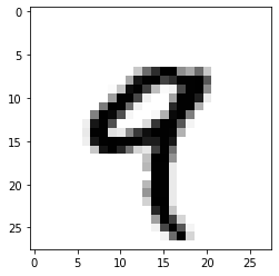
Displaying the fourth digit

Using Matplotlib to show the 4th of the 60000 training examples

import matplotlib.pyplot as plt
digit = train_images[4]
plt.imshow(digit, cmap=plt.cm.binary)
plt.show()

#and its label is:
train_labels[4]

9

Manipulating tensors in NumPy

different views or sub-parts of a tensor/array are called slices

my_slice = train_images[10:100] 
#note this doesn't include the element at 100
my_slice.shape

(90, 28, 28)

#this is the same operation as before but more detailed
#the colon says include everything in the dimension the colon is located

my_slice = train_images[10:100, :, :]
my_slice.shape

(90, 28, 28)

#you could also just say everything from 0 to 27 for those last two dimensions

my_slice = train_images[10:100, 0:28, 0:28]
my_slice.shape

(90, 28, 28)

#matplotlib counts from the top-left to bottom-right horizantally
#The following would select the bottom right of the images
my_slice = train_images[:, 14:, 14:]

#this would crop the middle square of the images
#the negative indices indicate a relative distance from the end of the tensor
my_slice = train_images[:, 7:-7, 7:-7]

The notion of data batches

By convention, the first axis/dimension of the tensor keeps each individual training example or sample

The first axis can also be called the batch dimension

Deep learning models won’t train on the entirety of the dataset at once. They do it on small batches of the training set at a time.

Here we train on the first 128 images

batch_size = 128
batch = train_images[:batch_size]

Here we train on the next 128 images

batch = train_images[batch_size:(batch_size*2)]

This is generalizable for the nth batch:

n = 3
batch = train_images[batch_size * n:batch_size * (n + 1)]

Real-world examples of data tensors

• Vectors (samples, features)
• Timeseries (samples, timesteps, features)
• Images (samples, height, width, channels)
• Video (samples,frames,height,width,channels)

Vector data

• we technically reshaped the MNIST dataset from a Rank-3 dataset to Rank-2 when we changed the 28x28 to 784 size.
• The cars dataset with each car being a sample and information about make, model, year, mpg, engine size, etc. Same for the iris dataset

Timeseries data or sequence data

• time axis is always the second axis by convention

• an example would be a dataset of stock prices throughout the day or year

Image data

• images have samples, height, width, and three color channels

• 200 color images of size 100x100 could be stored in a tensor of shape (200, 100, 100, 3)

• By convention, the color channel either comes first after the sample dimension or last - most datasets carry the color channel last.

Video data

• A set of 10 movie clips, each 30 seconds long, sample 10 times per second, and sized 128x256, could be represented with a tensor of shape (10, 300, 128, 256, 3).

The gears of neural networks: tensor operations

• All input transformations can be reduced to a few different tensor operations/functions

The first example neural net we created was the dense layer:

keras.layers.Dense(512, activation="relu")

The dense layer is performed with the following function:

output = relu(dot(input, W) + b)

There’s three operations going on here:

1. Dot product of input tensor and tensor “W”

Quick dot product reference: $\begin{bmatrix} 1 & 2
3 & 4
10 & 0
\end{bmatrix} * [3, -1] = [[1,2][3,-1]+[3,4][3,-1]+[10,0]*[3,-1]$ $=[1, 5, 30]$

1. Adding that matrix with vector b (the bias)

$[1, 5, 30]+[3, 12, -32]=[4, 17, -2]$

1. Performing a relu operation - max(x,0) and stands for “rectified linear unit”

relu($[4, 17, -2]$)=$[4, 17, 0]$

Element-wise operations

The following functions use nested for loops to go through each element of their tensors and apply relu and addition of two vectors.

This shows how the math is performed for these operations but our numerical libraries can perform them much faster via vectorized and parallel operations than these for loops ever could.

The difference in time is shown for the final two examples, the first has been vectorized using the numpy library, the second uses the for loops. These times add up significantly for large training sets.

My machine ran the numbers in 0.0040 seconds versus the for loop of 1.77 seconds. A speedup factor of 442.5!

def naive_relu(x):
    assert len(x.shape) == 2
    x = x.copy()
    for i in range(x.shape[0]):
        for j in range(x.shape[1]):
            x[i, j] = max(x[i, j], 0)
    return x

def naive_add(x, y):
    assert len(x.shape) == 2
    assert x.shape == y.shape
    x = x.copy()
    for i in range(x.shape[0]):
        for j in range(x.shape[1]):
            x[i, j] += y[i, j]
    return x

import time

x = np.random.random((20, 100))
y = np.random.random((20, 100))

t0 = time.time()
for _ in range(1000):
    z = x + y
    z = np.maximum(z, 0.)
print("Took: {0:.4f} s".format(time.time() - t0))

Took: 0.0030 s

t0 = time.time()
for _ in range(1000):
    z = naive_add(x, y)
    z = naive_relu(z)
print("Took: {0:.2f} s".format(time.time() - t0))

Took: 1.83 s

Broadcasting

When vectors don’t share the same shape, smaller shape will be broadcast across the larger one and reused.

import numpy as np
X = np.random.random((32, 10))
y = np.random.random((10,))

y = np.expand_dims(y, axis=0) #y becomes a (1,10) tensor

Y = np.concatenate([y] * 32, axis=0) #new Y for broadcasting

def naive_add_matrix_and_vector(x, y):
    assert len(x.shape) == 2
    assert len(y.shape) == 1
    assert x.shape[1] == y.shape[0]
    x = x.copy()
    for i in range(x.shape[0]):
        for j in range(x.shape[1]):
            x[i, j] += y[j]
    return x

#This function can now operate on the variables X and our new Y

import numpy as np
x = np.random.random((64, 3, 32, 10))
y = np.random.random((32, 10))
z = np.maximum(x, y)

#This broadcasts y multiple times to compare to x across it's dimensions

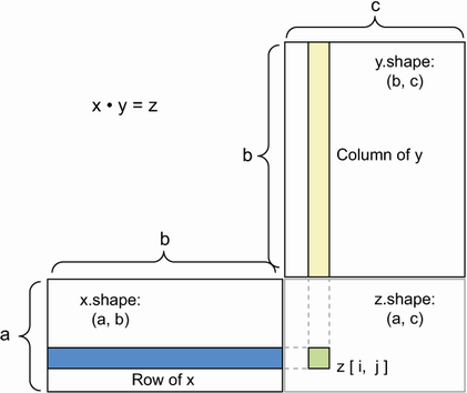
Tensor product (dot product)

• for two tensors to be multiplied, they must share the same size for their inner dimensions i.e. a (3,2)•(2,1) will result in a (3,1) vector but you can’t flip them and perform (2,1)•(3,2) because the 1 and 3 don’t match.

#Implementing a dot product in numpy

x = np.random.random((32,))
y = np.random.random((32,))
z = np.dot(x, y)

def naive_vector_dot(x, y):
    assert len(x.shape) == 1
    assert len(y.shape) == 1
    assert x.shape[0] == y.shape[0]
    z = 0.
    for i in range(x.shape[0]):
        z += x[i] * y[i]
    return z

def naive_matrix_vector_dot(x, y):
    assert len(x.shape) == 2
    assert len(y.shape) == 1
    assert x.shape[1] == y.shape[0]
    z = np.zeros(x.shape[0])
    for i in range(x.shape[0]):
        for j in range(x.shape[1]):
            z[i] += x[i, j] * y[j]
    return z

def naive_matrix_vector_dot(x, y):
    z = np.zeros(x.shape[0])
    for i in range(x.shape[0]):
        z[i] = naive_vector_dot(x[i, :], y)
    return z

def naive_matrix_dot(x, y):
    assert len(x.shape) == 2
    assert len(y.shape) == 2
    assert x.shape[1] == y.shape[0]
    z = np.zeros((x.shape[0], y.shape[1]))
    for i in range(x.shape[0]):
        for j in range(y.shape[1]):
            row_x = x[i, :]
            column_y = y[:, j]
            z[i, j] = naive_vector_dot(row_x, column_y)
    return z

Following rules and shapes apply for dot products of tensors of higher dimensions:

(a, b, c, d) • (d,) → (a, b, c)

(a, b, c, d) • (d, e) → (a, b, c, e)

Tensor reshaping

train_images = train_images.reshape((60000, 28 * 28))

x = np.array([[0., 1.],
             [2., 3.],
             [4., 5.]])
x.shape

(3, 2)

x = x.reshape((6, 1))
x

array([[0.],
       [1.],
       [2.],
       [3.],
       [4.],
       [5.]])

x = np.zeros((300, 20))
x = np.transpose(x) #exchange rows for columns
x.shape

(20, 300)

Geometric interpretation of tensor operations

All tensor ops can be represented as a transformation in a geomtric space.

Nasa has a good explanation about vector addition

• Vector addition translates one vector in the direction of the other.

$\begin{bmatrix} Horizontal Factor
Vertical Factor
\end{bmatrix} + \begin{bmatrix} x
y
\end{bmatrix}$

• Vector rotation of an angle can be accomplished via dot product

$\begin{bmatrix} cos(\theta) & -sin(\theta)
sin(\theta) & cos(\theta)
\end{bmatrix} • \begin{bmatrix} x
y
\end{bmatrix}$

• Scaling accomplished via vertical and horizontal scaling

$\begin{bmatrix} Horizontal Factor & 0
0 & Vertical Factor
\end{bmatrix} • \begin{bmatrix} x
y
\end{bmatrix}$

• Linear Transform - a dot product with an arbitrary matrix - this includes scaling and rotation in two specific cases

• Affine Transforms combine a linear transform with translation and is the most general.

Wikipedia has an excellent reference of different matrix operations for completing affine geometric transformations

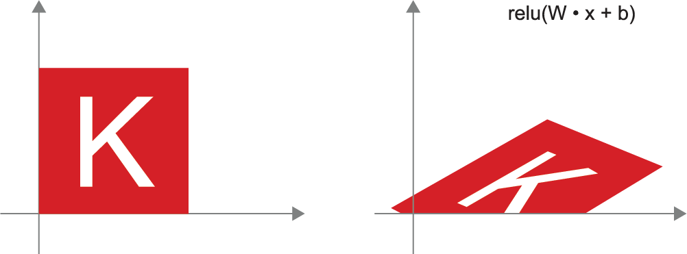
Since this is the most generic, it follows the format of $y = W • x + b$

Why are activation functions necessary?

A Dense layer without an activation function is an affine layer!

Without activation functions, each layer of a dense layer could be combined into a single affine transform. By adding the activation functions, we get much more non-linear transformations and expand the possibilities of data representation with much more potential.

A geometric interpretation of deep learning

• An intuitive explanation of deep learning is to crumple two different colored pieces of paper into a ball, and the transformations are a series of movements of the paper to flatten them out so they can be re-separated. Machine learning applies this but in much higher dimensional feature space than the 3D example of a crumpled paper ball.

The engine of neural networks: gradient-based optimization

Dense layer applies the function of $y = relu(W • x + b)$

x would be the input data, and W and b are the trainable parameters, commonly called the weights and biases.

When training a network, these values start randomly but the process of gradient optimization pushes those initial parameters to something more useful based on the goal and feedback.

A loop is required for this training to occur:

1. Get training examples with their targets
2. Run the model on the training examples to get predictions
3. Calculate the difference or loss between targets and predictions
4. Update the weights and biases of the model to slightly reduce the loss

Steps 1 through 3 are relatively trivial - 1 reads the data stored, 2 is our series of relu functions on the affine transformations, and 3 is a simple difference between the two.

But step four is the complicated part, we want to update all the parameters all at once to make this efficient. Operations research methods would hold everything constant and move one parameter and see how it affected the loss by redoing step 2 and 3 but to run it forward twice to check which way the parameter should be adjusted for a single parameter among thousands or millions would be ridiculously inefficient. To do this properly, we’re going to learn about gradient descent.

What’s a derivative?

• Given a continuous function, the slope of the function at any point is the derivative. It gives the rate of change of the function at any point. For a line, this is a trivial constant because it’s rate of change is constant. For the $x^2$ function, the function of its function is $2x$

• Even if the derivative isn’t linear, we can always perform a first-order approximation of the derivative at any point in x with a linear approximation of the derivative. This is useful for telling us the direction of the function x and magnitude.

• So if we have an optimization function and we’re looking for the value of x to minimize the loss, we just need to adjust x in the opposite direction of the current derivative. If the slope is negative, move it in the positive direction, and the amount of movement is proportional to the magnitude of the derivative.

Derivative of a tensor operation: the gradient

• gradients are the generalization of the concept of derivatives to function that take tensors as inputs.

• If $W_0$ is the tensor of initial weights, then the gradient will be a tensor indicating the direction of steepest ascent of $loss value = f(W)$ around $W_0$. Any partial derivative is the slope of $f$ in any specific direction.

Therefore, we can update our weights with the simple equation $W_1 = W_0 - step*grad(f(W_0), W_0)$

where $step$ is a scaling factor, usually designated with alpha $\alpha$

This process will lower you on the function curve and reduce your loss.

Alpha is required due to the loss only being approximated close to $W_0$ so we don’t want to wander too far from our initial location.

Stochastic gradient descent (SGD)

In neural nets, the loss function will be a minimum when the gradient is 0. Not every 0 is the global minimum but the global minimum will have a gradient of 0. For lower order polynomial functions, this value could be calculated directly, however, for neural nets, the order of magnitude are in the thousands or millions and are intractable for direct computation. (At least while we don’t have quantum calculation capabilities for tunneling directly to the answer.)

• Adagrad and RMSprop are common optimizers for implementing gradient descent with momentum

• If the learning rate is too small, the solution won’t converge quickly, if it’s too large, the solution will be overshot.

• True SGD computes the error one training example at a time, batch SGD updates after going over every single training example. A good compromise for efficiency is mini-batch SGD where one uses a reasonable number of examples and update based on their combined error.

• Momentum takes into account, not only the current gradient, but the previous gradients as well.

Nominal implementation:

past_velocity = 0. 
momentum = 0.1
while loss > 0.01:
    w, loss, gradient = get_current_parameters()
    velocity = past_velocity * momentum - learning_rate * gradient
    w = w + momentum * velocity - learning_rate * gradient
    past_velocity = velocity
    update_parameter(w)

Chaining derivatives: The Backpropagation algorithm

• The Backpropagation algorithm gives us a way to use gradient for the loss function of our neural nets and update the weights.

The chain rule

• Each simple tensor operation (relu, dot product, addition) has another simple known derivative. We use the chain rule to combine these operations into a single operation to find the overall derivative.

For a given function fg(x) where fg(x) is defined as f(g(x)), the chain rule states that the derivative or gradient of the new combined function grad(f(g(x),x) == grad(f(g(x)),g(x)) * grad(g(x), x)

In pseudocode form, for four functions nested together:

def fghj(x):
    x1 = j(x)
    x2 = h(x1)
    x3 = g(x2)
    y = f(x3)
    return y
 
grad(y, x) == (grad(y, x3) * grad(x3, x2) *
               grad(x2, x1) * grad(x1, x))

Automatic differentiation with computation graphs

• A computation graph is a data structure showing a directed acyclic graph of operations.

Our two-layer network computation graph:

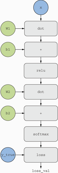
• They allow us to treat computations as data

• Modern libraries carryout automatic differentiation to take the created structure of the neural net and automatically compute the gradient based on the derivatives of the parts. It’s a hard problem that’s been simplified by modern tools.

• If you’d really like to dive into the math of how backpropogation works, consider this example and the following geogebra file

The gradient tape in TensorFlow

• Tensorflow’s implementation of automatic differentiation

#works with scalers

import tensorflow as tf
x = tf.Variable(0.)
with tf.GradientTape() as tape:
    y = 2 * x + 3
grad_of_y_wrt_x = tape.gradient(y, x)
grad_of_y_wrt_x

<tf.Tensor: shape=(), dtype=float32, numpy=2.0>

#works with tensor operations

x = tf.Variable(tf.random.uniform((2, 2)))
with tf.GradientTape() as tape:
    y = 2 * x + 3
grad_of_y_wrt_x = tape.gradient(y, x)
grad_of_y_wrt_x

<tf.Tensor: shape=(2, 2), dtype=float32, numpy=
array([[2., 2.],
       [2., 2.]], dtype=float32)>

# Also works with list of variables

W = tf.Variable(tf.random.uniform((2, 2)))
b = tf.Variable(tf.zeros((2,)))
x = tf.random.uniform((2, 2))
with tf.GradientTape() as tape:
    y = tf.matmul(x, W) + b
grad_of_y_wrt_W_and_b = tape.gradient(y, [W, b])
grad_of_y_wrt_W_and_b

[<tf.Tensor: shape=(2, 2), dtype=float32, numpy=
 array([[0.16477036, 0.16477036],
        [1.1502832 , 1.1502832 ]], dtype=float32)>,
 <tf.Tensor: shape=(2,), dtype=float32, numpy=array([2., 2.], dtype=float32)>]

Looking back at our first example

#input data

(train_images, train_labels), (test_images, test_labels) = mnist.load_data()
train_images = train_images.reshape((60000, 28 * 28))
train_images = train_images.astype("float32") / 255
test_images = test_images.reshape((10000, 28 * 28))
test_images = test_images.astype("float32") / 255

#our model

model = keras.Sequential([
    layers.Dense(512, activation="relu"),
    layers.Dense(10, activation="softmax")
])

#model compilation

model.compile(optimizer="rmsprop",
              loss="sparse_categorical_crossentropy",
              metrics=["accuracy"])

#training step

model.fit(train_images, train_labels, epochs=5, batch_size=128)

Epoch 1/5
469/469 [==============================] - 2s 3ms/step - loss: 0.2527 - accuracy: 0.9270
Epoch 2/5
469/469 [==============================] - 1s 3ms/step - loss: 0.1029 - accuracy: 0.9696
Epoch 3/5
469/469 [==============================] - 2s 3ms/step - loss: 0.0690 - accuracy: 0.9790
Epoch 4/5
469/469 [==============================] - 2s 3ms/step - loss: 0.0502 - accuracy: 0.9844
Epoch 5/5
469/469 [==============================] - 2s 3ms/step - loss: 0.0382 - accuracy: 0.9887





<keras.callbacks.History at 0x21976c28730>

Note that each iteration over the entire training set is called an epoch

Reimplementing our first example from scratch in TensorFlow

• Not implementing backpropagation or basic tensor operations

A simple Dense class

import tensorflow as tf

class NaiveDense:
    def __init__(self, input_size, output_size, activation):
        self.activation = activation

        #Create a matrix, W, of shpae (input_size, output_size),
        #Initialized with random values
        w_shape = (input_size, output_size)
        w_initial_value = tf.random.uniform(w_shape, minval=0, maxval=1e-1)
        self.W = tf.Variable(w_initial_value)

        #Create a vector, b, of shape (output_size,) initialized with zeros
        b_shape = (output_size,)
        b_initial_value = tf.zeros(b_shape)
        self.b = tf.Variable(b_initial_value)

    #Create capability for a forward pass
    def __call__(self, inputs):
        return self.activation(tf.matmul(inputs, self.W) + self.b)

    #Add the capability of retrieving the layer's weights
    @property
    def weights(self):
        return [self.W, self.b]
    
    

A simple Sequential class

This class will chain the layers together

class NaiveSequential:
    def __init__(self, layers):
        self.layers = layers

    #Calls underlying layers on the inputs, in order. 
    def __call__(self, inputs):
        x = inputs
        for layer in self.layers:
           x = layer(x)
        return x
    
    #easily keep track of the layer's paramters
    @property
    def weights(self):
       weights = []
       for layer in self.layers:
           weights += layer.weights
       return weights

#Now we can create a mockup of a Keras model

model = NaiveSequential([
    NaiveDense(input_size=28 * 28, output_size=512, activation=tf.nn.relu),
    NaiveDense(input_size=512, output_size=10, activation=tf.nn.softmax)
])
assert len(model.weights) == 4

A batch generator

For iterating over the MNIST data, we create a batch generator

import math

class BatchGenerator:
    def __init__(self, images, labels, batch_size=128):
        assert len(images) == len(labels)
        self.index = 0
        self.images = images
        self.labels = labels
        self.batch_size = batch_size
        self.num_batches = math.ceil(len(images) / batch_size)

    def next(self):
        images = self.images[self.index : self.index + self.batch_size]
        labels = self.labels[self.index : self.index + self.batch_size]
        self.index += self.batch_size
        return images, labels

Running one training step

Here, we’ll update the weights of the model after running it on one batch of data. We need to:

• Compute the predictions of the model for the images in the batch.
• Compute the loss value for these predictions, given the actual labels.
• Compute the gradient of the loss with regard to the model’s weights.
• Move the weights by a small amount in the direction opposite to the gradient.

We will use the TensorFlow GradientTape object

def one_training_step(model, images_batch, labels_batch):
    #Run the "forward pass"
    #(Computer the model's predictions under a GradientTape scope)
    with tf.GradientTape() as tape:
        predictions = model(images_batch)
        per_sample_losses = tf.keras.losses.sparse_categorical_crossentropy(
            labels_batch, predictions)
        average_loss = tf.reduce_mean(per_sample_losses)
        
    #Compute the gradient of the loss with regard to the weights
    #The output gradients is a list where each entry corresponds to a
    #weight from the model.weights list
    gradients = tape.gradient(average_loss, model.weights)
    
    #Update the weights using the gradients using the next function 
    update_weights(gradients, model.weights)
    return average_loss

learning_rate = 1e-3

#The simplest way to update the weights is to subtract
#gradient * learning_rate from each weight

def update_weights(gradients, weights):
    for g, w in zip(gradients, weights):
        w.assign_sub(g * learning_rate)

#But this is never done by hand
#Instead, we use an optimzer instance

from tensorflow.keras import optimizers

optimizer = optimizers.SGD(learning_rate=1e-3)

def update_weights(gradients, weights):
    optimizer.apply_gradients(zip(gradients, weights))

The full training loop

def fit(model, images, labels, epochs, batch_size=128):
    for epoch_counter in range(epochs):
        print(f"Epoch {epoch_counter}")
        batch_generator = BatchGenerator(images, labels)
        for batch_counter in range(batch_generator.num_batches):
            images_batch, labels_batch = batch_generator.next()
            loss = one_training_step(model, images_batch, labels_batch)
            if batch_counter % 100 == 0:
                print(f"loss at batch {batch_counter}: {loss:.2f}")

from tensorflow.keras.datasets import mnist
(train_images, train_labels), (test_images, test_labels) = mnist.load_data()

train_images = train_images.reshape((60000, 28 * 28))
train_images = train_images.astype("float32") / 255
test_images = test_images.reshape((10000, 28 * 28))
test_images = test_images.astype("float32") / 255

#use our training class made from scratch!
fit(model, train_images, train_labels, epochs=10, batch_size=128)

Epoch 0
loss at batch 0: 5.94
loss at batch 100: 2.25
loss at batch 200: 2.22
loss at batch 300: 2.11
loss at batch 400: 2.23
Epoch 1
loss at batch 0: 1.94
loss at batch 100: 1.89
loss at batch 200: 1.84
loss at batch 300: 1.73
loss at batch 400: 1.84
Epoch 2
loss at batch 0: 1.62
loss at batch 100: 1.58
loss at batch 200: 1.52
loss at batch 300: 1.44
loss at batch 400: 1.52
Epoch 3
loss at batch 0: 1.36
loss at batch 100: 1.34
loss at batch 200: 1.25
loss at batch 300: 1.23
loss at batch 400: 1.28
Epoch 4
loss at batch 0: 1.16
loss at batch 100: 1.15
loss at batch 200: 1.05
loss at batch 300: 1.06
loss at batch 400: 1.11
Epoch 5
loss at batch 0: 1.02
loss at batch 100: 1.01
loss at batch 200: 0.91
loss at batch 300: 0.94
loss at batch 400: 0.99
Epoch 6
loss at batch 0: 0.90
loss at batch 100: 0.90
loss at batch 200: 0.80
loss at batch 300: 0.85
loss at batch 400: 0.90
Epoch 7
loss at batch 0: 0.82
loss at batch 100: 0.82
loss at batch 200: 0.72
loss at batch 300: 0.78
loss at batch 400: 0.83
Epoch 8
loss at batch 0: 0.76
loss at batch 100: 0.75
loss at batch 200: 0.66
loss at batch 300: 0.72
loss at batch 400: 0.78
Epoch 9
loss at batch 0: 0.70
loss at batch 100: 0.70
loss at batch 200: 0.61
loss at batch 300: 0.67
loss at batch 400: 0.74

Evaluating the model

predictions = model(test_images)
predictions = predictions.numpy()
predicted_labels = np.argmax(predictions, axis=1)
matches = predicted_labels == test_labels
print(f"accuracy: {matches.mean():.2f}")

accuracy: 0.82

Summary

• Tensors form the foundation of modern machine learning systems. They come in various flavors of dtype, rank, and shape.

• You can manipulate numerical tensors via tensor operations (such as addition, tensor product, or element-wise multiplication), which can be interpreted as encoding geometric transformations. In general, everything in deep learning is amenable to a geometric interpretation.

• Deep learning models consist of chains of simple tensor operations, parameterized by weights, which are themselves tensors. The weights of a model are where its “knowledge” is stored.

• Learning means finding a set of values for the model’s weights that minimizes a loss function for a given set of training data samples and their corresponding targets.

• Learning happens by drawing random batches of data samples and their targets, and computing the gradient of the model parameters with respect to the loss on the batch. The model parameters are then moved a bit (the magnitude of the move is defined by the learning rate) in the opposite direction from the gradient. This is called mini-batch stochastic gradient descent.

• The entire learning process is made possible by the fact that all tensor operations in neural networks are differentiable, and thus it’s possible to apply the chain rule of derivation to find the gradient function mapping the current parameters and current batch of data to a gradient value. This is called backpropagation.

• Two key concepts you’ll see frequently in future parts are loss and optimizers. These are the two things you need to define before you begin feeding data into a model.

  1. The loss is the quantity you’ll attempt to minimize during training, so it should represent a measure of success for the task you’re trying to solve.
  2. The optimizer specifies the exact way in which the gradient of the loss will be used to update parameters: for instance, it could be the RMSProp optimizer, SGD with momentum, and so on.