Deep Learning Part 3 - Keras & Tensorflow
Introduction to Keras and TensorFlow
This part covers
- How TensorFlow and Keras work individually and together
- Setting up a deep learning workspace
- An overview of how core deep learning concepts translate to Keras and TensorFlow
This is Part 3 of a companion notebook for Deep Learning with Python, Second Edition. The original notebook only contained runnable code blocks and section titles and omitted everything else. I have added my notes and comments to the book for more significant learning and reference capabilities.
#Running a custom runtime with anaconda

#(base) conda install nb_conda_kernels
# conda create --name deep-learning
# conda activate deep-learning
# conda install ipykernel
# conda install tensorflow==2.6 keras==2.6

#Here in Jupyter, menu>Kernel>Change kernel>conda env:deep-learning
What’s TensorFlow?
Expands on capabilities of NumPy
- Automatically computes the gradient of any differentiable expression
- Runs on CPUs, GPUs, and TPUs (Tensor Processing Units) for processing parallelism
- TensorFlow computation can be distributed across machines.
- Runtimes can be exported to other programs making deployment easier.
TensorFlow (TF) is more of a platform than a library. Components include
- TF-Agents for reinforcement-learning
- TFX ML workflow management
- TF Serving for production deployment
- TF Hub is a repository of pre-trained models
What’s Keras?
Convenient API built on TF.
- Consistent and simple workflows
- Easy to learn and very productive
- Lots of top-end researchers use it
- You can treat it like Scikit-learn at the top level or deep in the details as if it were NumPy.
- Supportable regardless of where you’re at in your professional development career trajectory
- Similar to Python in how flexible it is
Keras and TensorFlow: A brief history
- Developed almost at the same time but Keras came out eight months before TF. It was originally made for Theano - a precursor to TF.
- Along with TF, Keras was used as the front end for other tensor libraries including MXNet (Amazon), and CNTK (Microsoft) but those are now either out of development or are only used at their respective companies.
Setting up a deep-learning workspace
- Run these operations on an NVIDIA GPU, not a CPU. Image tasks are extremely slow on CPUs.
Options: - Buy your own GPU - GPU instances on Google Cloud or Amazon Web Services (AWS EC2) - Run the free GPU on Colaboratory but this isn’t good for anything beyond basic operations.
Jupyter notebooks can use the cloud instances relatively easily.
But GPU costs can add up quickly so probably best to purchase your own GPU.
Running on Windows is not recommended - Use Unix. It seems like a hassle but in the long run, a lot of time will be saved. Set up a Ubuntu dual boot or use the Windows Subsystem for Linux
Jupyter notebooks: The preferred way to run deep-learning experiments
- Jupyter notebooks (which is how this notebook was originally created prior to being converted for the web) mixes the capabilities to execute code along with markdown for rich text-editing for annotations. These notebooks also allow parts of the program to be broken up so if a mistake is made, the entirety of the code before doesn’t have to be re-run.
Using Colaboratory
Website for creating Jupyter notebooks.
It is recommended for basic experiments and duplicating the code in this series of deep learning content. Provides GPU and TPU runtimes.
- https://colab.research.google.com
- Contains text and code cells
- It’s incredibly easy to produce code and generate results
- In Colab, adding the “!” command allows a shell command e.g.
!pip install package_name
- In Colab, select Runtime>Change Runtime and select GPU for hardware acceleration.
- TPU is another option but it requires manual setup in the code beforehand. We should go over this in more detail in [[Deep Learning Part 13]]
First steps with TensorFlow
Training a neural net requires:
- Low level tensor manipulation
- Tensors/variables
- Tensor operations (
relu,matmul) - Backprop
- High level deep learning concepts
- We use Keras APIs
- Layers combined into a model
- Loss Function
- Optimizer
- Metrics
- Training Loop
Constant tensors and variables
Tensors need to be created with some initial value. This could be a constant like the ones and zeros or a random distributions below.
All-ones or all-zeros tensors
import tensorflow as tf
x = tf.ones(shape=(2, 1))
print(x)
tf.Tensor(
[[1.]
 [1.]], shape=(2, 1), dtype=float32)
x = tf.zeros(shape=(2, 1))
print(x)
tf.Tensor(
[[0.]
 [0.]], shape=(2, 1), dtype=float32)
Random tensors
x = tf.random.normal(shape=(3, 1), mean=0., stddev=1.)
print(x)
tf.Tensor(
[[-0.7330572 ]
 [ 0.52187616]
 [-0.77484965]], shape=(3, 1), dtype=float32)
x = tf.random.uniform(shape=(3, 1), minval=0., maxval=1.)
print(x)
tf.Tensor(
[[0.00733709]
 [0.25006843]
 [0.0751164 ]], shape=(3, 1), dtype=float32)
NumPy arrays are assignable
But TF tensors are NOT assignable, they’re constant.
import numpy as np
x = np.ones(shape=(2, 2))
x[0, 0] = 0.
print(x)
[[0. 1.]
 [1. 1.]]
x = tf.ones(shape=(2, 2))
x[0, 0] = 0.
---------------------------------------------------------------------------

TypeError                                 Traceback (most recent call last)

~\AppData\Local\Temp/ipykernel_6472/3106594083.py in <module>
      1 x = tf.ones(shape=(2, 2))
----> 2 x[0, 0] = 0.


TypeError: 'tensorflow.python.framework.ops.EagerTensor' object does not support item assignment
Creating a TensorFlow variable
You have to be able to update the state of a model which is made up of a set of tensors. To making something assignable - we use variables. tf.Variable is used for items with a modifiable state. You do have to provide an initial value though.
v = tf.Variable(initial_value=tf.random.normal(shape=(3, 1)))
print(v)
<tf.Variable 'Variable:0' shape=(3, 1) dtype=float32, numpy=
array([[ 1.6343002 ],
       [-0.10996494],
       [ 0.42412648]], dtype=float32)>
Assigning a value to a TensorFlow variable
v.assign(tf.ones((3, 1)))
<tf.Variable 'UnreadVariable' shape=(3, 1) dtype=float32, numpy=
array([[1.],
       [1.],
       [1.]], dtype=float32)>
Assigning a value to a subset of a TensorFlow variable
v[0, 0].assign(3.)
<tf.Variable 'UnreadVariable' shape=(3, 1) dtype=float32, numpy=
array([[3.],
       [1.],
       [1.]], dtype=float32)>
Using assign_add and assign_sub
#equivalent to += and -= in python
v.assign_add(tf.ones((3, 1)))
<tf.Variable 'UnreadVariable' shape=(3, 1) dtype=float32, numpy=
array([[4.],
       [2.],
       [2.]], dtype=float32)>
Tensor operations: Doing math in TensorFlow
A few basic math operations
a = tf.ones((2, 2))
b = tf.square(a) #takes the square
c = tf.sqrt(a) #takes the square root
d = b + c #element-wise addition of two tensors
e = tf.matmul(a, b) #dot product of two tensors
e *= d #multiple two tensors element-wise
Each operation is performed at that time and you can see the current results. This is eager execution
A second look at the GradientTape API
- TF can perform operations NumPy can’t - prime example is GradentTape for any differentiable expression with respect to any of its inputs.
Using the GradientTape
input_var = tf.Variable(initial_value=3.)
with tf.GradientTape() as tape:
   result = tf.square(input_var)
gradient = tape.gradient(result, input_var)
print(gradient)
tf.Tensor(6.0, shape=(), dtype=float32)
Using GradientTape with constant tensor inputs
Only trainable variables are tracked by default but TF’s gradient tape can have any arbitrary tensor as input.
With a constant tensor, we have to manually mark it for tracking with tape.watch()
This is to save resources and not track everything with respect to everything.
input_const = tf.constant(3.)
with tf.GradientTape() as tape:
   tape.watch(input_const)
   result = tf.square(input_const)
gradient = tape.gradient(result, input_const)
print(gradient)
tf.Tensor(6.0, shape=(), dtype=float32)
Using nested gradient tapes to compute second-order gradients
Gradient tapes can also take the gradient of a gradient.
Basic physics is a good example of a use here - gradient of position is speed, the gradient of speed is acceleration.
time = tf.Variable(0.)
with tf.GradientTape() as outer_tape:
    with tf.GradientTape() as inner_tape:
        position =  4.9 * time ** 2
    speed = inner_tape.gradient(position, time)
acceleration = outer_tape.gradient(speed, time)

print(acceleration)
tf.Tensor(9.8, shape=(), dtype=float32)
An end-to-end example: A linear classifier in pure TensorFlow
Tensors, variables, tensor operations, and gradient computing are enough to build an ML model based on gradient descent.
A common interview question is to implement a linear classifier from scratch in TF.
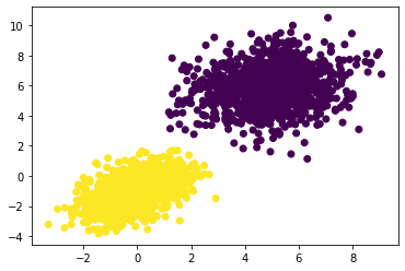
First, some synthetic data - two classes of points in a 2D plane.
Generating two classes of random points in a 2D plane
num_samples_per_class = 1000
positive_samples = np.random.multivariate_normal(
    mean=[0, -1],
    cov=[[1, 0.5],[0.5, 1]],
    size=num_samples_per_class)
negative_samples = np.random.multivariate_normal(
    mean=[5, 6],
    cov=[[2, 0.25],[0.25, 2]],
    size=num_samples_per_class)
Stacking the two classes into an array with shape (2000, 2)
inputs = np.vstack((negative_samples, positive_samples)).astype(np.float32)
Generating the corresponding targets (0 and 1)
#use 0's for negative and 1's for positive
targets = np.vstack((np.zeros((num_samples_per_class, 1), dtype="float32"),
                     np.ones((num_samples_per_class, 1), dtype="float32")))
Plotting the two point classes
import matplotlib.pyplot as plt
plt.scatter(inputs[:, 0], inputs[:, 1], c=targets[:, 0])
plt.show()
Creating the linear classifier variables
A linear classifier is an affine transformation (prediction = W • input + b) trained to minimize the square of the difference between predictions and the targets.
input_dim = 2 #inputs will be 2D points
output_dim = 1 # output predictions will be close to 0 for 0, and 1 if class 1
W = tf.Variable(initial_value=tf.random.uniform(shape=(input_dim, output_dim)))
b = tf.Variable(initial_value=tf.zeros(shape=(output_dim,)))
The forward pass function
def model(inputs):
    return tf.matmul(inputs, W) + b
The mean squared error loss function
def square_loss(targets, predictions):
    per_sample_losses = tf.square(targets - predictions) #contains per sample loss scores
    return tf.reduce_mean(per_sample_losses) #averages per-sample losses to a single scaler
The training step function
This is the critical step - completing a training step. This will update the weights of W and b to minimize the loss of this data.
learning_rate = 0.03

def training_step(inputs, targets):

    #forward pass, inside the scope of a gradient tape
    with tf.GradientTape() as tape:
        predictions = model(inputs)
        loss = square_loss(predictions, targets)

    #Get the gradient of the loss with respect to W and b
    grad_loss_wrt_W, grad_loss_wrt_b = tape.gradient(loss, [W, b])

    #Update the weights based on the new gradient
    W.assign_sub(grad_loss_wrt_W * learning_rate)
    b.assign_sub(grad_loss_wrt_b * learning_rate)
    return loss
The batch training loop
Although not normal practice, we’ll conduct batch training using all 2000 samples instead of mini-batch sampling using random batches of 128. This will take longer but updates to the weights will also be larger so we can use a larger learning rate.
for step in range(150):
    loss = training_step(inputs, targets)
    if step %10 == 0:
        print(f"Loss at step {step}: {loss:.4f}")
Loss at step 0: 16.3559
Loss at step 10: 3.2022
Loss at step 20: 0.7233
Loss at step 30: 0.2193
Loss at step 40: 0.0972
Loss at step 50: 0.0579
Loss at step 60: 0.0412
Loss at step 70: 0.0328
Loss at step 80: 0.0283
Loss at step 90: 0.0258
Loss at step 100: 0.0245
Loss at step 110: 0.0237
Loss at step 120: 0.0233
Loss at step 130: 0.0231
Loss at step 140: 0.0229
predictions = model(inputs)
plt.scatter(inputs[:, 0], inputs[:, 1], c=predictions[:, 0] >= 0.5)
plt.show()

x = np.linspace(-2, 8, 100) #100 regularly spaced numbers between our min and max range

#rearrange w1*x+w2*y+b= 0.5 for the discriminating line that splits 1 vs 0.
y = - W[0] /  W[1] * x + (0.5 - b) / W[1]

plt.plot(x, y, "-r") #plot as a red line

plt.scatter(inputs[:, 0], inputs[:, 1], c=predictions[:, 0] >= 0.5) #plot the original data too
plt.show()
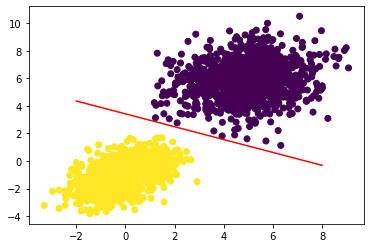
We’ve developed a 2D line separating the two classes of data!
Let’s put all the code into one place for easy reference:
def model(inputs):
return tf.matmul(inputs, W) + b
def square_loss(targets, predictions):
per_sample_losses = tf.square(targets - predictions) #contains per sample loss scores
return tf.reduce_mean(per_sample_losses) #averages per-sample losses to a single scaler
def training_step(inputs, targets):
#forward pass, inside the scope of a gradient tape
with tf.GradientTape() as tape:
predictions = model(inputs)
loss = square_loss(predictions, targets)
#Get the gradient of the loss with respect to W and b
grad_loss_wrt_W, grad_loss_wrt_b = tape.gradient(loss, [W, b])
#Update the weights based on the new gradient
W.assign_sub(grad_loss_wrt_W * LEARNING_RATE)
b.assign_sub(grad_loss_wrt_b * LEARNING_RATE)
return loss
NUM_SAMPLES_PER_CLASS = 1000
LEARNING_RATE = 0.03
positive_samples = np.random.multivariate_normal(
mean=[0, -1],
cov=[[1, 0.5],[0.5, 1]],
size=NUM_SAMPLES_PER_CLASS)
negative_samples = np.random.multivariate_normal(
mean=[5, 6],
cov=[[2, 0.25],[0.25, 2]],
size=NUM_SAMPLES_PER_CLASS)
inputs = np.vstack((negative_samples, positive_samples)).astype(np.float32)
#use 0's for negative and 1's for positive
targets = np.vstack((np.zeros((NUM_SAMPLES_PER_CLASS, 1), dtype="float32"),
np.ones((NUM_SAMPLES_PER_CLASS, 1), dtype="float32")))
input_dim = 2 #inputs will be 2D points
output_dim = 1 # output predictions will be close to 0 for 0, and 1 if class 1
W = tf.Variable(initial_value=tf.random.uniform(shape=(input_dim, output_dim)))
b = tf.Variable(initial_value=tf.zeros(shape=(output_dim,)))
for step in range(150):
loss = training_step(inputs, targets)
if step %10 == 0:
print(f"Loss at step {step}: {loss:.4f}")
predictions = model(inputs)
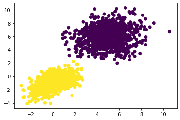
#plotting
import matplotlib.pyplot as plt
plt.scatter(inputs[:, 0], inputs[:, 1], c=targets[:, 0])
plt.show()
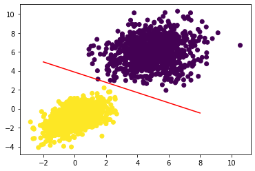
#plot predictions
x = np.linspace(-2, 8, 100) #100 regularly spaced numbers between our min and max range
#rearrange w1*x+w2*y+b= 0.5 for the discriminating line that splits 1 vs 0.
y = - W[0] / W[1] * x + (0.5 - b) / W[1]
plt.plot(x, y, "-r") #plot as a red line
plt.scatter(inputs[:, 0], inputs[:, 1], c=predictions[:, 0] >= 0.5) #plot the original data too
plt.show()
Loss at step 0: 33.1227
Loss at step 10: 14.3233
Loss at step 20: 6.2363
Loss at step 30: 2.7306
Loss at step 40: 1.2053
Loss at step 50: 0.5402
Loss at step 60: 0.2497
Loss at step 70: 0.1226
Loss at step 80: 0.0669
Loss at step 90: 0.0424
Loss at step 100: 0.0316
Loss at step 110: 0.0268
Loss at step 120: 0.0246
Loss at step 130: 0.0237
Loss at step 140: 0.0233
Anatomy of a neural network: Understanding core Keras APIs
We now know how to implement a simple linear classifier and a basic neural network from Part 2. It’s now time to learn the Keras API.
Layers: The building blocks of deep learning
The layer is the fundamental building block and data structure of a neural network. It processes data by taking in tensor input(s), applying some operation(s), and producing output(s). Most layers contain information about the state of the layer which is held in the weights associated with that layer. These weights contain the transformations and representations of the inherent knowledge held within the neural net.
-
Vector data can be represented well by rank-2 tensors of shape
(samples, features)and often processed by densely connected (fully connected) layers. -
Sequence data, with rank-3 tensors
(samples, timesteps, features), is typically processed with recurrent layers. Common recurrent layers includeLSTMor 1D convolution layers (Conv1D). -
Image data in Rank-4 tensors is usually processed with 2D convolutional layers (
Conv2D)
Layers are the lego bricks of deep learning and Keras provides the implementation of those bricks.
The base Layer class in Keras
Everything in the Keras API is centered on the Layer class. Most items are either a layer or interact with a layer.
A Layer holds both the computation of the forward pass of the layer along with information about its state held within its weights. Weights are normally created when the layer is initially constructed with the __init__() function or with the build() function. Computations are defined with the call() function.
A Dense layer implemented as a Layer subclass
In Part 2, the NaiveDense layer was implemented with W and b. This is the same layer in Keras.
from tensorflow import keras

#All Keras layers inherit from the base Layer class
class SimpleDense(keras.layers.Layer):

    def __init__(self, units, activation=None):
        super().__init__()
        self.units = units
        self.activation = activation

    #Weight creation is accomplished via the build() method
    def build(self, input_shape):
        #automatic shape inference based on tensor input
        input_dim = input_shape[-1]

        #add_weight() is a shortcut method for creating weights
        #It's also possible to create standalone variables
        #and assign them as layer attributes
        #An example would be
        #    self.W = tf.Variable(tf.random.uniform(w_shape))
        self.W = self.add_weight(shape=(input_dim, self.units),
                                 initializer="random_normal")
        self.b = self.add_weight(shape=(self.units,),
                                 initializer="zeros")

    #We define the forward pass computation in the call() method
    def call(self, inputs):
        y = tf.matmul(inputs, self.W) + self.b
        if self.activation is not None:
            y = self.activation(y)
        return y
This layer can now be used like a function with a TF tensor as input.
#Create an instance of the previously defined layer
my_dense = SimpleDense(units=32, activation=tf.nn.relu)

#Create test inputs
input_tensor = tf.ones(shape=(2, 784))

#Call the layer on the inputs like a function
output_tensor = my_dense(input_tensor)

print(output_tensor.shape)
(2, 32)
call() and build() needed to be present in the SimpleDense class so the state can be created just in time.
Automatic shape inference: Building layers on the fly
Any layer with compatibility with another layer can be chained together, (like the earlier referenced Lego bricks). Compatibility refers specifically to the shape of the incoming tensor and the shape of the output. To make things more flexible, many layers will infer the shape needed to give this compatibility.
Our previous NaiveDense Dense layer required input size explicitly stated which makes things tedious.
This would have resulted in code looking like this:
model = NaiveSequential([
    NaiveDense(input_size=784, output_size=32, activation="relu"),
    NaiveDense(input_size=32, output_size=64, activation="relu"),
    NaiveDense(input_size=64, output_size=32, activation="relu"),
    NaiveDense(input_size=32, output_size=10, activation="softmax")
])
SimpleDense weights are created automatically via the build() method, which is called via __call__() the first time the layer is also called.
This is also why the call() method was defined instead of __call__() directly.
The base Layer __call__() method is defined by:
def __call__(self, inputs):
    if not self.built:
         self.build(inputs.shape)
         self.built = True
    return self.call(inputs)
Therefore, when the layer is initially called, it takes the input tensor, grabs its shape, feeds it to the build method, adds the attribute the layer has been built, and performs the contents of the call() method.
Not defining the layer in terms of its input tensor would also make it incredibly difficult for layers with more complex output such as a shape that’s defined as (batch, input_ size * 2 if input_size % 2 == 0 else input_size * 3)
Here’s an example of shape inference:
from tensorflow.keras import layers
layer = layers.Dense(32, activation="relu")
#first layer will have 32 outputs
#Keras will automatically build
#the layers to match the shape of the incoming layer
from tensorflow.keras import models
from tensorflow.keras import layers
model = models.Sequential([
    layers.Dense(32, activation="relu"),
    layers.Dense(32)
])
Our previous example becomes much neater with automatic shape inference:
model = keras.Sequential([
    SimpleDense(32, activation="relu"),
    SimpleDense(64, activation="relu"),
    SimpleDense(32, activation="relu"),
    SimpleDense(10, activation="softmax")
])
__call__() also handles eager vs. graph execution which has more detail in [[Part 7]] and input masking [[Part 11]].
The biggest takeaway is The forward pass needs to be put in the call() method
From layers to models
The entire model used in a deep-learning use case is made up of a graph of layers. These are wrapped in Keras with the Model class.
Sequential is a subclass of Model.
Other common model topologies include:
- Two-branch networks
- Multi-head networks
- Residual connections
A Transformer architecture (responsible for significant advances in natural language processing ([[NLP]])) is a reasonably involved architecture that looks like the figure below:
![]()
You can build models directly by subclassing the Model class but the preferred method is using the Functional API. [[Part 7]] will cover both approaches
The topology of a model defines a hypothesis space. Machine learning is searching for useful representations of some input data. By choosing a network topology you constrain your space of possibilities to a specific series of tensor operations, mapping input data to output data.
To learn from data, one must make assumptions about it. These assumptions define what can be learned. The structure of your hypothesis space—the architecture of your model is extremely important. It encodes the assumptions you make about your problem. For instance, if you’re working on a two-class classification problem, you are assuming that your two classes are linearly separable.
Picking the right network architecture is more of an art than a science. The next few parts will teach you explicit principles for building neural networks. They’ll also help you develop intuition as to what works or doesn’t work for specific problems. You’ll build a solid intuition about what type of model architectures work for different kinds of problems.
The “compile” step: Configuring the learning process
If you are training a neural network, you need to choose the loss function (objective function), optimizer, and metrics that you want to monitor during training and validation. The loss function is the quantity that will be minimized during training, while the optimizer determines how the network will be updated. Metrics measures success and the model won’t directly optimize for these parameters.
Use compile() and fit() to start training the model.
You can also write your own training loops.
compile() configures the training process - it takes the optimizer, loss, and list of metrics.
#Defines a linear classifier
model = keras.Sequential([keras.layers.Dense(1)])

model.compile(optimizer="rmsprop", #specify optimizer
              loss="mean_squared_error", #loss by name
              metrics=["accuracy"]) #list of metrics
The strings above are shortcuts to Python objects, they provide a convenient shortcut instead of going about using the following syntax:
model.compile(optimizer=keras.optimizers.RMSprop(),
              loss=keras.losses.MeanSquaredError(),
              metrics=[keras.metrics.BinaryAccuracy()])
This method of writing out functions is useful if you want custom losses, metrics, or wanted to pass an argument to one of the objects such as the learning rate for the optimizer.
Available Options:
Optimizers:
- SGD (with or without momentum)
- Adagrad
- RMSprop
- Adam
Losses:
- CategoricalCrossentropy
- SparseCategoricalCrossentropy
- BinaryCrossentropy
- MeanSquaredError
- KLDivergence
- CosineSimilarity
Metrics:
- CategoricalAccuracy
- SparseCategoricalAccuracy
- BinaryAccuracy
- AUC
- Precision
- Recall
Picking a loss function
Choosing the right loss function for the right problem is extremely important. If the objective doesn’t fully correlate with success for the task at hand, your network will end up doing things you may not have wanted. All neural networks you build will be ruthless in lowering their loss function.
Common rules exist for classification, regression, and sequence prediction. Common rules of thumb will be explored in further detail but for two-class classification, we use binary crossentropy, and categorical crossentropy for many-class classification. Generally, only new research problems require new loss functions.
Understanding the fit() method
fit() implements training itself.
Key arguments:
-
Data - inputs and targets - to train on. Can be either NumPy array or TF
Dataset -
Number of epochs (How many times the training loop should iterate over the data passed)
-
Batch size for mini-batch gradient descent
Calling fit() with NumPy data
history = model.fit(
    inputs, #input examples as NumPy array
    targets, #corresponding targets as NumPy array
    epochs=5, #iterate over the dataset 5 times
    batch_size=128 #iterate over the data in chunks of 128
)
Epoch 1/5
16/16 [==============================] - 0s 665us/step - loss: 7.6743 - binary_accuracy: 0.0200
Epoch 2/5
16/16 [==============================] - 0s 600us/step - loss: 6.8800 - binary_accuracy: 0.0155
Epoch 3/5
16/16 [==============================] - 0s 600us/step - loss: 6.2362 - binary_accuracy: 0.0135
Epoch 4/5
16/16 [==============================] - 0s 600us/step - loss: 5.6408 - binary_accuracy: 0.0105
Epoch 5/5
16/16 [==============================] - 0s 533us/step - loss: 5.0885 - binary_accuracy: 0.0085
fit() returns a History object which contains history - a dictionary mapping keys such as "loss" and metrics to their per-epoch values.
history.history
{'loss': [7.674332618713379,
  6.879999160766602,
  6.236242771148682,
  5.640758037567139,
  5.088471412658691],
 'binary_accuracy': [0.019999999552965164,
  0.01549999974668026,
  0.013500000350177288,
  0.010499999858438969,
  0.008500000461935997]}
Monitoring loss and metrics on validation data
We need to remember the goal isn’t specifically to minimize our loss for the model - we want to find a model that generalizes well, especially for information the model hasn’t seen before. This improved performance on the training set and poor on the test data is called overfitting and is equivalent to the model memorizing all the input data.
For this reason, it’s standard practice to keep a subset of the data as our validation data. You can keep this data by adding the validation_data argument.
Using the validation_data argument
model = keras.Sequential([keras.layers.Dense(1)])
model.compile(optimizer=keras.optimizers.RMSprop(learning_rate=0.1),
              loss=keras.losses.MeanSquaredError(),
              metrics=[keras.metrics.BinaryAccuracy()])

#shuff hte inputs and targets using random indices to prevent
#only one class from being in the validation data
indices_permutation = np.random.permutation(len(inputs))
shuffled_inputs = inputs[indices_permutation]
shuffled_targets = targets[indices_permutation]

#We want to keep 30% of the training data for validation
#They'll be completely excluded from training
#and used to compute validation loss and metrics
num_validation_samples = int(0.3 * len(inputs))
val_inputs = shuffled_inputs[:num_validation_samples]
val_targets = shuffled_targets[:num_validation_samples]
training_inputs = shuffled_inputs[num_validation_samples:]
training_targets = shuffled_targets[num_validation_samples:]

model.fit(
    #Use our normal training data for sculpting the weights
    training_inputs,
    training_targets,
    epochs=5,
    batch_size=16,
    #Here we use the validation data for losses and metrics
    validation_data=(val_inputs, val_targets)
)
Epoch 1/5
88/88 [==============================] - 0s 2ms/step - loss: 0.4252 - binary_accuracy: 0.8607 - val_loss: 1.0908 - val_binary_accuracy: 0.9733
Epoch 2/5
88/88 [==============================] - 0s 793us/step - loss: 0.2215 - binary_accuracy: 0.9086 - val_loss: 1.1732 - val_binary_accuracy: 0.9633
Epoch 3/5
88/88 [==============================] - 0s 736us/step - loss: 0.2042 - binary_accuracy: 0.8750 - val_loss: 0.1097 - val_binary_accuracy: 1.0000
Epoch 4/5
88/88 [==============================] - 0s 747us/step - loss: 0.2228 - binary_accuracy: 0.8864 - val_loss: 0.0217 - val_binary_accuracy: 1.0000
Epoch 5/5
88/88 [==============================] - ETA: 0s - loss: 0.0184 - binary_accuracy: 1.000 - 0s 724us/step - loss: 0.2105 - binary_accuracy: 0.8964 - val_loss: 0.0246 - val_binary_accuracy: 1.0000


<keras.callbacks.History at 0x1f0586794f0>
We can also do this via a post-training call for the model to evaluate new data:
loss_and_metrics = model.evaluate(val_inputs, val_targets, batch_size=128)
5/5 [==============================] - 0s 750us/step - loss: 0.0246 - binary_accuracy: 1.0000
Inference: Using a model after training
After training a model, using the model for predictions is called inference. It always takes significantly less computational power than the initial model training.
Use the predict() method for conducting this.
Using predict() on our validation data with the linear model gives scalar scores that correlate to the predictions for each input sample.
predictions = model.predict(val_inputs, batch_size=128)
print(predictions[:10])
[[-0.07636255]
 [-0.11595923]
 [ 0.98395574]
 [ 0.18966657]
 [ 0.03606886]
 [ 0.822527  ]
 [ 0.91361773]
 [ 0.07334584]
 [ 0.09287828]
 [ 1.0012345 ]]
Summary
- TensorFlow is an industry-strength numerical computing framework that can run on CPU, GPU, or TPU. It can automatically compute the gradient of any differentiable expression, it can be distributed to many devices, and it can export programs to various external runtimes.
- Keras is the standard API for doing deep learning with TensorFlow.
- Key TensorFlow objects include tensors, variables, tensor operations, and the gradient tape.
- The central class of Keras is the Layer. A layer encapsulates some weights and some computation. Layers are assembled into models.
- Before you start training a model, you need to pick an optimizer, a loss, and some metrics, which you specify via the model.compile() method.
- To train a model, you can use the fit() method, which runs mini-batch gradient descent for you. You can also use it to monitor your loss and metrics on validation data, a set of inputs that the model doesn’t see during training.
- Once your model is trained, you use the model.predict() method to generate predictions on new inputs. (Inference)
To Do
- Insert Link for [[Deep Learning Part 13]]
- Insert Link for [[Part 7]]
- Insert Link for [[Part 11]]
- [[Part 7]] links x2